
Some time ago I saw an interesting post in a R related group on LinkedIn. It was from Michael Piccirilli and he wrote something about his new package Rlinkedin. I was really impressed by his work and so I decided to write a blog post about it.
Get the package
The package is currently just available via GitHub. But thanks to devtools it is not a problem to install it.
|
1 2 3 4 5 |
require(devtools) install_github("mpiccirilli/Rlinkedin") require(Rlinkedin) |
Authenticate with LinkedIn
In the next step we have to connect to the LinkedIn API via oAuth 2.0. You have two possibilities in the Rlinkedin package.
You can just use
|
1 |
in.auth <- inOAuth() |
to use a default API key for getting LinkedIn data.
Or:
You can use your own application and application credentials to connect to the API.
Therefore you have to create an application on LinkedIn. Go on https://www.linkedin.com/secure/developer and log in with your LinkedIn account. Then click on “Add new Application”.
![]()
On the next page you can see app settings. Just set them as you can see on the following screenshots:
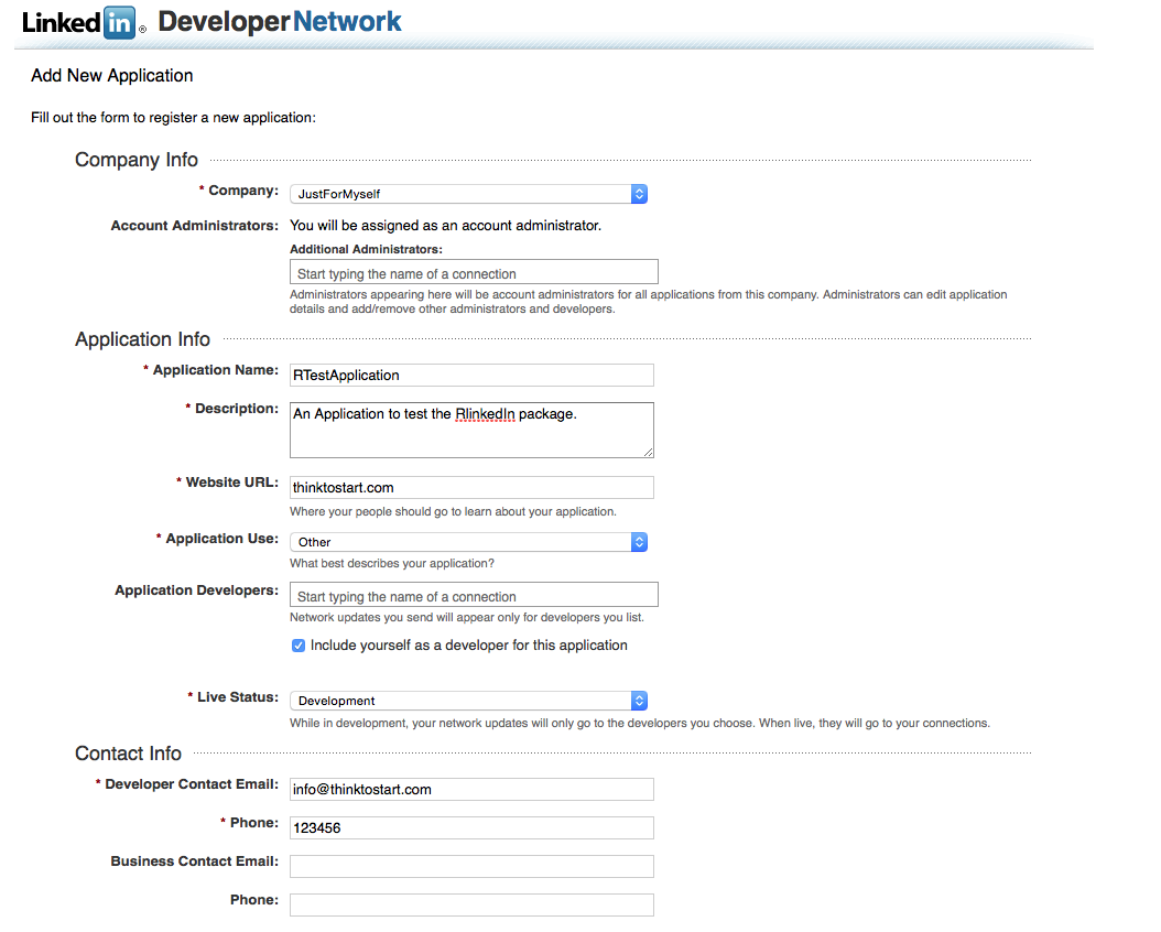
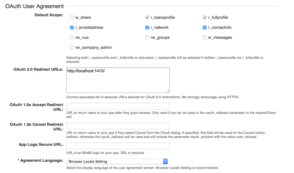
Then click on “Add application” and you get forwarded to your app´s credentials. Switch back to R and set the following variables:
|
1 2 3 |
app_name <- "XXX" consumer_key <- "XXX" consumer_secret <- "XXX" |
Then you can authenticate with:
|
1 |
in.auth <- inOAuth(app_name, consumer_key, consumer_secret) |
After a successful authentication you start to get some data.
Analyze LinkedIn with R
Michael created a nice overview of the different functions on the package´s GitHub page. So I will just show you here a small sample analysis.
First, lets download all your connections with:
|
1 |
my.connections <- getMyConnections(in.auth) |
This creates a data frame with all available information about your connections. For our analysis we will get the column “industry” which is the industry the person is working in. We will use it to create a small word cloud.
|
1 |
text <- toString(my.connections$industry) |
We will then transform this text with some standard word cloud to a nice looking industry overview:
|
1 2 3 4 5 6 7 8 9 10 11 12 13 14 15 16 17 18 19 20 21 22 23 24 25 26 27 28 29 30 31 32 33 34 35 36 37 38 |
clean.text <- function(some_txt) { some_txt = gsub("(RT|via)((?:\\b\\W*@\\w+)+)", "", some_txt) some_txt = gsub("@\\w+", "", some_txt) some_txt = gsub("[[:punct:]]", "", some_txt) some_txt = gsub("[[:digit:]]", "", some_txt) some_txt = gsub("http\\w+", "", some_txt) some_txt = gsub("[ \t]{2,}", "", some_txt) some_txt = gsub("^\\s+|\\s+$", "", some_txt) some_txt = gsub("amp", "", some_txt) # define "tolower error handling" function try.tolower = function(x) { y = NA try_error = tryCatch(tolower(x), error=function(e) e) if (!inherits(try_error, "error")) y = tolower(x) return(y) } some_txt = sapply(some_txt, try.tolower) some_txt = some_txt[some_txt != ""] names(some_txt) = NULL return(some_txt) } clean_text = clean.text(text) tweet_corpus = Corpus(VectorSource(clean_text)) tdm = TermDocumentMatrix(tweet_corpus, control = list(removePunctuation = TRUE,stopwords = stopwords("english"), removeNumbers = TRUE, tolower = TRUE)) #install.packages(c("wordcloud","tm"),repos="http://cran.r-project.org") library(wordcloud) m = as.matrix(tdm) #we define tdm as matrix word_freqs = sort(rowSums(m), decreasing=TRUE) #now we get the word orders in decreasing order dm = data.frame(word=names(word_freqs), freq=word_freqs) #we create our data set wordcloud(dm$word, dm$freq, random.order=FALSE, colors=brewer.pal(8, "Dark2")) #and we visualize our data |
This will create a word cloud like the following:
