Build a SPAM filter with R

You can find the complete code on github:

https://github.com/JulianHill/R-Tutorials/blob/master/spam_class_r.r

 

Introduction:

The topic Machine Learning gets more and more important. The number of data sources grows everyday and it makes it hard to get insights out of this huge amount of data.
This increases the need for machine learning algorithms.

Our example focuses on building a spam detection engine. So our system should be able to classify a given e-mail as spam or not-spam

If you never heard of machine learning or supervised and unsupervised learning before you should take a look at some basic machine learning tutorials like

inside-bigdata.com: Data Science 101 Machine Learning Part 1 or

www.realtechsupport.org: Machine Learning 

Our example describes a supervised machine learning problem. And so we can use a SVM. I chose it because it shows the power of machine learning with R very good and also delivers pretty good results on our problem. But I will also write a post about solving this problem with Random Forests as especially in the last time more and more people use this algorithm.

If you want to read about how to select a model you can take a look here: http://blog.echen.me/2011/04/27/choosing-a-machine-learning-classifier/

What is a Support Vector Machine?:

Let´s take a look at what wikipedia says about SVMs: An SVM model is a representation of the examples as points in space, mapped so that the examples of the separate categories are divided by a clear gap that is as wide as possible. New examples are then mapped into that same space and predicted to belong to a category based on which side of the gap they fall on. http://en.wikipedia.org/wiki/Support_vector_machine

So in general the SVM algorithm tries to separate the data with a gap that is as wide as possible. It does so with the help of vectors which define hyperplanes.

The Data for our SPAM model

Our purpose is to build a spam detection engine. This is a classification problem as the outcome should be either 0 for no spam and 1 for spam. So if the SVM analyses a single email it will return a 0 or a 1.
We get our dataset from the UCI Machine Learning Repository  https://archive.ics.uci.edu/ml/datasets/Spambase
This so called “Spambase” dataset contains real data examples. So the author analysed real emails.
The dataset contains 57 attributes or features. These consist of:

At this point it is not important for us how the author of the dataset found out that these words are important.

It also contains attributes which show the number of certain chars in the Email like

And also 3 attributes focusing on capital letters.

They are about the average length uninterrupted sequence of capital letters, the length of longest uninterrupted sequence and the total number of capital letters in the e-mail.

And of course the last attribute which denoted whether the e-mail was considered spam (1) or not (0).

Load the data to R

I copied the data to a csv file you can download here:

Just put it in your R working directory and load it with:

The data frame we just created does not have useful column names as they were not defined in the csv. This will be a problem as the SVM algorithm can handle names like the automatically created V1, V2 or so.

So we have to rename them properly. Therefore I also copied the attribute names and put them in a CSV file you can find here:

and load it with:

Then we just have to set this list as the names of our dataset data frame with:

In the next step we transform the y column, which is numeric at the moment, to factor values. If we would call the SVM function with a numeric output column it would automatically assume that we want to use a regression even if there are just two different variables in the dataset. Transforming this column to factor values makes the SVM to use a classification output.

The data actually consists of 4601 rows. So 4601 classified e-mails. These could be a little bit too much for our way to create a Support Vector Machine as I will explain later. But therefore we build it with a sample of our dataset based on 1000 e-mails

 

Build a SPAM filter with R

 

To create the SVM we need the caret package. This is like a layer on top of a lot of different classification and regression packages in R and makes them available through easy to use functions.

Let´s install some packages we need:

The kernlab package is the short form for Kernel-based Machine Learning Lab. It implements methods for classification, regression and more but on a deeper layer than caret. So it actually contains the algorithms we use with the caret package and also provides other useful functions I will talk about later.

We have to split our dataset in two parts: One we need to train the SVM model and one to actually test if it works.

The caret package provides a handy function for this task.

http://www.inside-r.org/packages/cran/caret/docs/createDataPartition

We can use it:

This uses the output column of your sample dataset and splits and returns a index of which row will be in the train set and which row will be in the train set. It tries to keep the distribution of 0 and 1 in the both datasets. Otherwise it could happen that one dataset mostly contain out of negative examples and the other one mostly out of positive examples.

To actually split the data we apply this index to our sample set with:

Now we use the doMC package we installed a few minutes ago.

This makes our R instance use 5 cores or at least how many your computer has. This increases the speed of our SVM calculation a lot. The caret package will look for a registered doMC and if it exists it will use it automatically.

Ok the next step is about finding the right tuning parameters for our SVM.

Therefore we use on the sigest function from the kernlab package to find the best sigma value and we create a TuneGrid with that.

 

So the SVM needs two parameters for the training process:

sigma and C

If you want to know what these parameters are exactly you can take a look at: http://feature-space.com/en/post65.html and http://stats.stackexchange.com/questions/31066/what-is-the-influence-of-c-in-svms-with-linear-kernel

The C parameter tells the SVM optimization how much you want to avoid misclassifying each training example. For large values of C, the optimization will choose a smaller-margin hyperplane if that hyperplane does a better job of getting all the training points classified correctly. Conversely, a very small value of C will cause the optimizer to look for a larger-margin separating hyperplane, even if that hyperplane misclassifies more points. For very tiny values of C, you should get misclassified examples, often even if your training data is linearly separable.

 

In the first step we estimate the sigma value and the grid combines the sigma value with all values we defined for C. The train function uses this grid to create for every combination a SVM and just keeps the one which performed best.

Train the SVM

This is probably the most important step. We train the SVM with the train() function of the caret package. This function can be used for all the models and algorithms in the caret package. We define which data we want to use and what method to create the model.

You can find a detailed list of the parameters of the train() function here:

http://www.inside-r.org/packages/cran/caret/docs/train

 Evaluation:

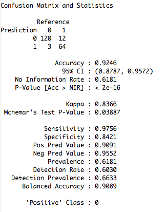
Now we created our model X. We can use this model to classify emails as spam or non-spam; so to perform a binary classification.

For the evaluation of the model we use the dataframe dataTest and the predict() function of the caret package. We exclude the last column of the dataframe which contents the label if the email is spam or no spam.

We save the predicted results in the variable pred and compare the results based on our model with the actual results in the last column of the dataTest dataframe.